|
|||||||||||||||||||||||||
|
|||||||||||||||||||||||||
| BeamLossPattern program for LHC collimation studies |
| |
| Contents 4. Features of BeamLossPattern 6. Source files and executables 7. Auxiliary programs (CountAbs, CleanInelastic, GetAperture) 8. Examples of simulation results 10. Updated aperture model for optics version V6.500 [May 2006] |
| |
| Why is it important to study beam losses? So far, the performance of the LHC collimation system has been studied by using approximate estimates of the transverse population of beam halo. The so-called cleaning inefficiency [1] (Ex.), calculated as the leackage rate of particles that escape from the cleaning insertions, is simulated by taking into account particle tracking throught the magnetic elements and scattering processing in the collimator jaws. The local cleaning inefficiency allows studying the performance of the collimation system, e.g. tolerances on various parameter of the LHC optics and of the collimator mechanics [ref. to RA, chamonix 2003]. Nevertheless, this approximated treatment does not allow one to predict the exact locations of losses around the ring, which is crucial, for example, to estimate the deposited energy on the superconducting magnets. In order to find out the precise locations of losses, one must check the trajectories of each halo particle and check if they hit the aperture walls somewhere in the machine. This requires (1) an accurate tracking of the particle trajectory and (2) a detailed aperture model of the full ring. The program BeamLossPattern has been developed to perform detailed beam loss studies for machines like the LHC. |
| |
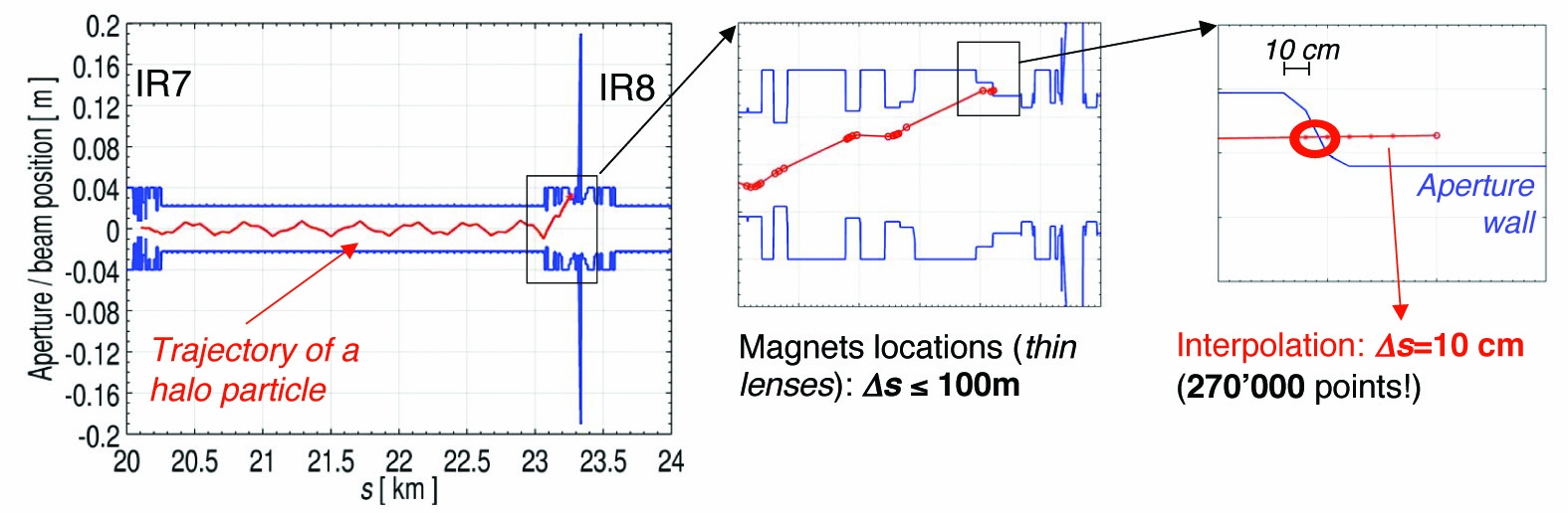
|
BeamLossPattern is a program that calculates the location of particle losses along an accelerator. It relies on an aperture model of the full machine and takes as an input the particle coordinate as a function of the longitudinal coordinate (referred to as particle trajectories). The figure below illustrates an example of trajectory of a lost particle. Locations of beam losses are identified with a spatial resolution of 10 centimetres. For the 27 km long LHC ring, this is equivalent to checking 270000 loss locations! This is achieved by interpolating trajectories between to consecutive lattice elements (typical distance up to > 100 m). The BeamLossPattern program has been optimized for the usage with the tracking tools developed for the LHC collimation studies (a new SixTrack version is used for collimation studies). For example, it can handle large input files (trajectory files of sizes up to 30GB are processed as a standard simulation campaign). However, the extension to other machines is trivial: one only needs to prodecu trajectories of halo particle with the correct input files format for BeamLossPattern (see below). It was decided to setup up a simulation tool for beam loss pattern studies independent on the tracking tool. The motivation for this choice is that checking the aperture within the tracking program with the required precision of <10 cm would slow down too much the simulation time. It is noted that the LHC collimation system is designed to provide cleaning inefficiency of the order of 1e-3 to 1e-4. Therefore, in order to accumulate decent statistics on the "few" lost particles, several million of input halo particles must be tracked. In addition, the fact of having an independent program
for beam loss studies has another advantage. For a give set of tracked
trajectories, studies for aperture misalignment, closed orbit, etc.
may be performed with many statistical seed without requiring tracking
simulations for every seed. This further optimizes the time required
for simulations. Example of BeamLossPattern: Trajectory
of a particle lost in an LHC interaction region (get
PDF file). |
| |
|
The aperture model is a crucial ingredient for producing reliable beam loss maps! Wrong aperture definition of some elements, empty spaces with no aperture defined or wrong locations of aperture bottlenecks can change completely the predictions of loss locations. The LHC aperture model has mostly been set by using that MADX interfaces with the LHC layout database. However, several aperture definitions required the preparation of dedicated MADX scripts in order to complement missing information on the database (see below). It is noted that the program BeamLossPattern is completely independent on MADX. MADX is only used to generate input files for the aperture program (aperture definitions versus longitudinal coordinate, survey files with the position of the design orbit, closed-orbit distortions, etc...). In particular, this means that the generated MADX scripts have not been conceived for MADX users: detailed MADX studies (e.g., particle tracking, APL aperture studies) might require different optimization such as positioning of aperture definition markers, definitions of aperture for specific elements, etc. Aperture files For the moment, the aperture model for the LHC optics version V6.5 (sequence) contains:
Known missing elements: Recombination chambers, position of vacuum chamber flanges of IR6 kickers. MADX sample job: sequence,
injection strength
file, lowb
strength file The input files for BeamLossPattern: (inj, lowb) Zipped file with all required input (uncompress with 'gtar -xvjf GenerateAperture.tgj') Remark: It is noted that the aperture
of collimators and protection devices are not
included in the aperture model of the ring. The reason for this
choice is that the treatment of these elements is carried out within
the tracking code, which provides directly the number of impacting
particles on the collimators and the locations of inelastic impacts
within the volume of the collimator jaws. The BeamLossPattern program does recognize square apertures and hence collimators can easily be modelled if needed. Collimator gap values can he found here. Aperture types accepted by the program (RECTELLIPSE notation, see MADX manual): Circle, square, ellipse, LHC beam screen, RaceTrack. |
| |
BeamLossPattern - some features Treatment of the design orbit position within the separation dipoles The LHC design orbit normaly passes throught the aperture centre of all elements. Some exceptions are represented by the separation dipoles, conventionally referred to and D1, D2, D3 and D4. These dipoles are installed at either side of the straight sections around the interaction points and are used to kick the beam in the same vacuum pipe (D1 and D2 magnets, experiment regions) and to increase the beam-beam separation (D3 and D4 magnets, RF, dump and cleaning regions). BeamLossPattern can misalign the aperture around the beam trajectory to take into account for the offset between aperture centre and circulating beam. This requires loading and external "survey file" with the corresponding offsets as a function of the longitudinal coordinate along the accelerator. Example scripts to generate such files are given below.
Treatment of the crossing angle/separation schemes Similarly to the previous case, separation and crossing schemes [ref to LHC design report] can also be taken into account. The main difference with respect to the orbit survey is that the crossing and separation kicker can be included in the tracking tools (this is indeed the case for SixTrack) and in this case it not necessary to add off-line the offsets to the particles' trajectories. An internal flag (_X_), set to .FALSE. as default, is available in BeamLossPattern to switch on and off this option. The inpu files with the information on the crossing/separation schemes are generated similarly to the survey files, as discussed below.
Saving the trajectories of lost particles It is possible to save the trajectories of all lost particles.
In order to save disk space, only the trajectory of the last turn
is recorded.
Calculation of the number of surviving turns BeamLossPattern calculates the number of surviving turns before the halo particles hit the aperture. This is given as a standard output in the last column of the beam loss files.
|
| |
BeamLossPattern users's manual Required inputs:
Command line (all the above inputs must be in the same directory): BeamLossPattern Energy Halo.File Output.Name Aperture.File Energy --------> "inj" or "lowb" (used to identify the survey file) Standard outputs The output files has basically the same format has the input halo file. The only difference is that the last column know gives the number of surviving turns for each particle, i.e. the number of turn between the interaction with the primary collimators and the turn when the particle is lost. Remarks (1) Format of halo file (example) The halo files generated by SixTrack contains the following 9
columns: For the program to function properly, it is mandatory that each halo particle is univocally identified by a particle
number, which must be between 0 and 30000 (Np parameter in
the source). This upper value can be changed in the source code. It is noted that the format of the numbers in the halo file is not important, provided that each line contains 9 "words". By default, the first line is a header and is disregarded in the analysis. (2) Survey files (3) Flags that can be set internally (require recompilation) -> See also here.
|
| |
|
Zipped file with code source and makefile: BeamLossPattern.tgz (Uncompress with 'gtar') Compiled executables:
|
| |
|
1) CountAbs (input naming conventions specific for LHC simultion setup) This program is used to count the number of "real" impacts
on the collmator jaws all around the ring. Particles that, according
to the SixTrack calculations, interact with the collimators might
instead have reached aperture bottlenecks before hitting
the collimators jaws. Therefore, these particles must be disregarded
in the counting of impacts/absorptions on the collimators. It is noted that the contribution of "fake" collimator impacts is very small because the collimation system is designed such that the collimator are the closet elements to the beam. Typically, a few percent of the total impacts at most are "fake". Nevertheless, with CountAbs it can now taken into account. Source.cpp (stand-alone code, just compile with 'g++') How to run it -The command line looks like "CountAbs
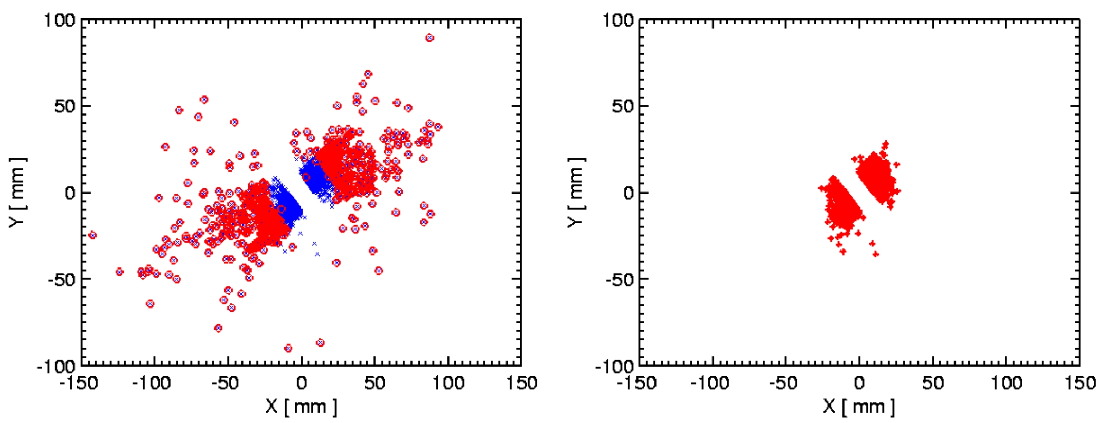
SeedNumber Halo Energy Optics" Default input names: Default output name: Input options: The SixTrack version with collimation can provide the locations of inelastic impacts of protons with the collimator jaws, which are used as an input for energy deposition studies. As discussed above, the SixTrack output can overestimate the number of impacts in a given collimator because it does not disregard the particles hitting the ring aperture before reaching the collimator (no aperture checks are carried out during the tracking). Similarly to CountAbs, CleanInelastic cleans up the "fake" inelastic impacts from the SixTrack output. Note that several input files are required to reconstruct the longitudinal position of the collimators in the sequence because of the collimator numbering used in SixTrack (which in principle can vary from run to run). Source.cpp (stand-alone code, just compile with 'g++') How to run it: "CleanInelastic Impact.file Loss.file CollPosition coll_summary.dat" Inputs: Outputs: impacts_fake.dat, impacts_real.dat Example of the usage of CleanInelastic:
trasnverse scatter plot of inelastic impacts at the first secondary
collimator of IR7 (TCSG.A6L7) before (left) and after (right) correction
of "fake" impacts (simulations at injection) [Get
EPS file].
For a given lattice and aperture model, this program produces an ascii files with the aperture every 10 cm all along the beam line. Aperture values are given at three different azimuthal angles: 0, pi/4 and pi/2. Source .cpp (compile with 'make GetAperture' - same makefile of BeamLossPattern) How to run it: "GetAperture ApertureModel.file" (e.g. "-> GetAperture allaper_inj_20050322.b1") Input: Aperture model input file, as it is used by BeamLossPattern |
| |
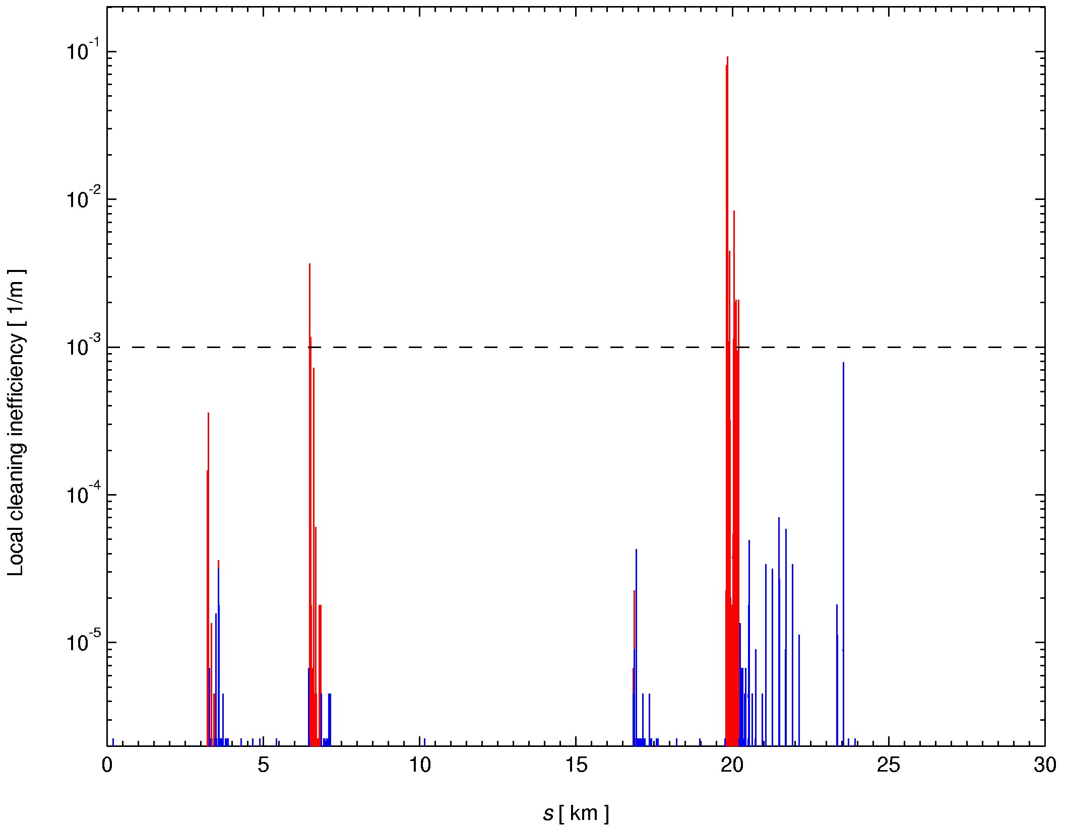
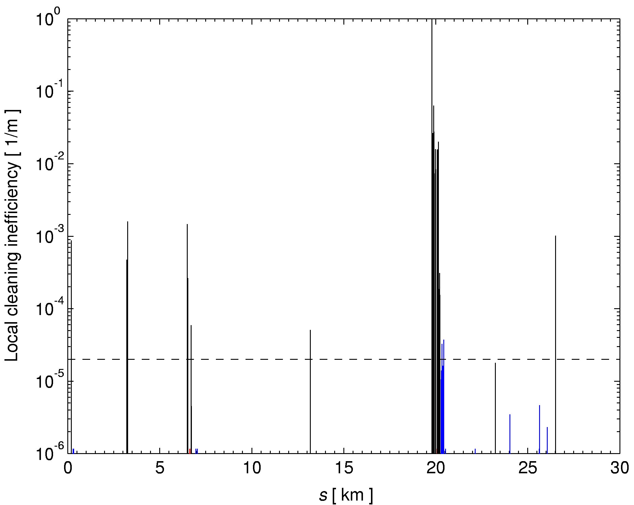
Examples of simulation results (preliminary) In the following plots, the losses are given in unit of local cleaning inefficiency. Loss maps at injection energy
(horizontal halo - 5000000 tracked particles).
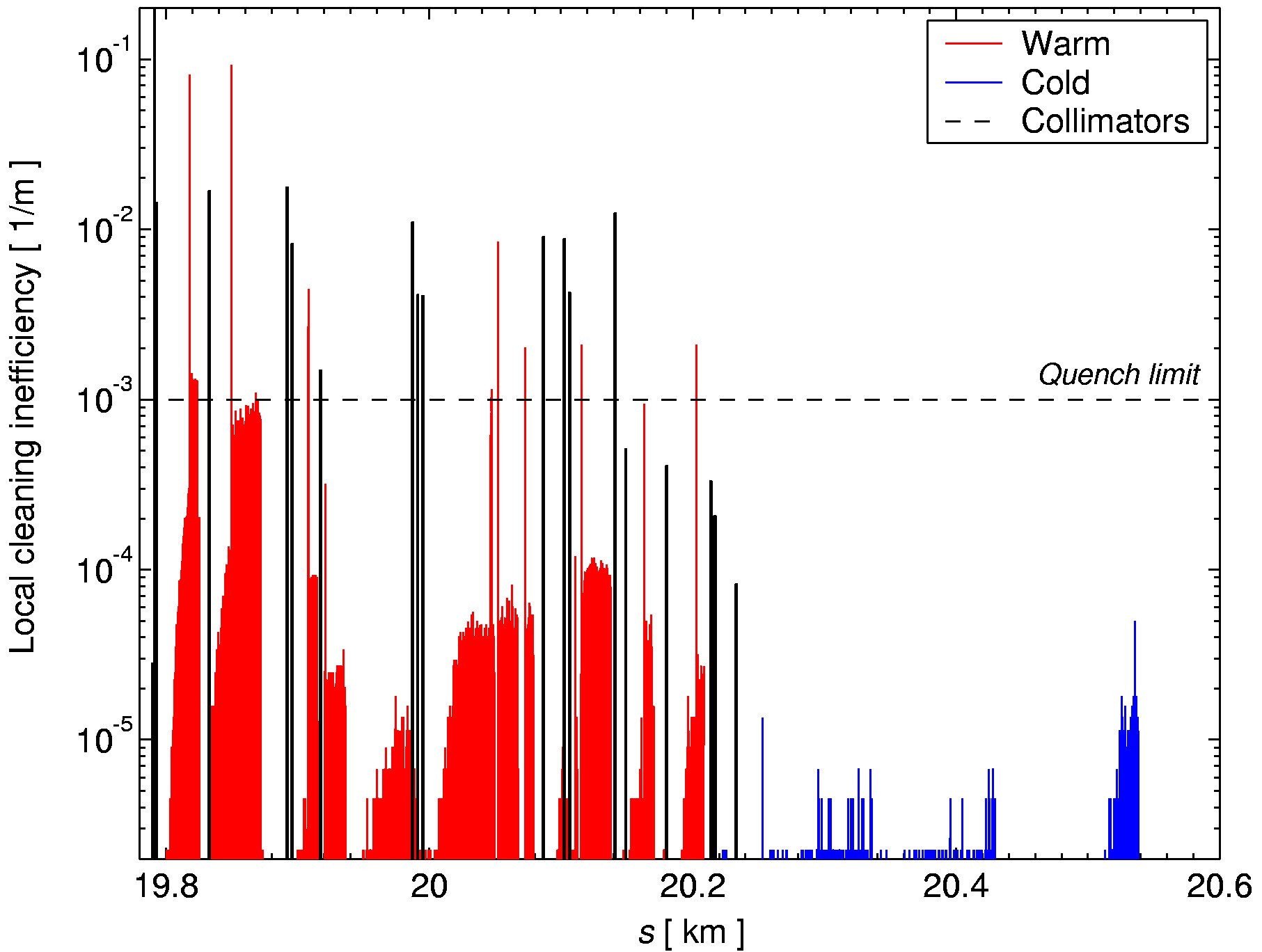
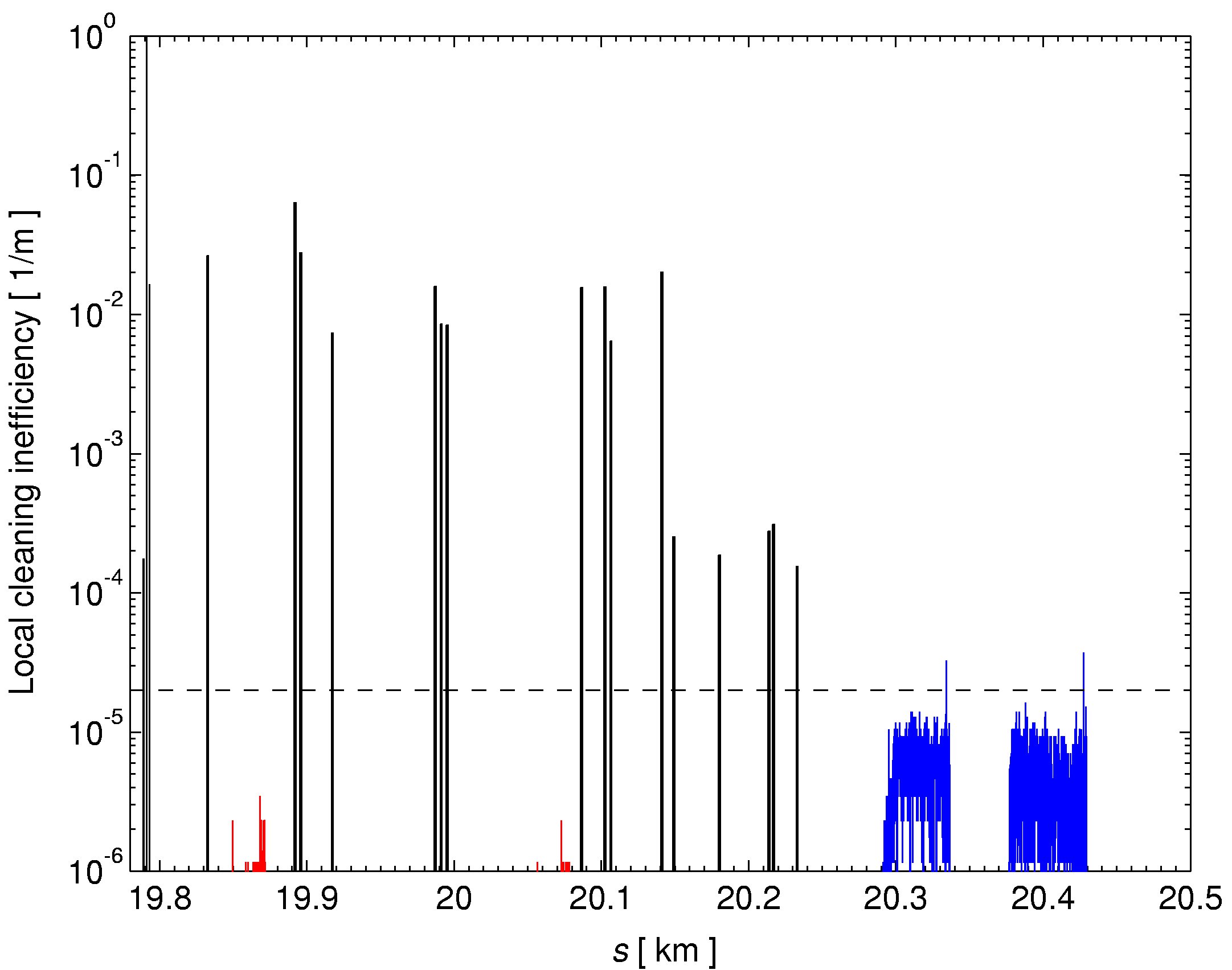
Losses at IR7 and downstream dispersion suppressor
(zoom of the above plot).
Loss maps at top energy, with all tertiary collimators
at their nominal settings (horizontal halo - 5000000 tracked
particles). Losses in IR7 and downstream
dispersion suppressor - 7 TeV(Zoom of the above plot).
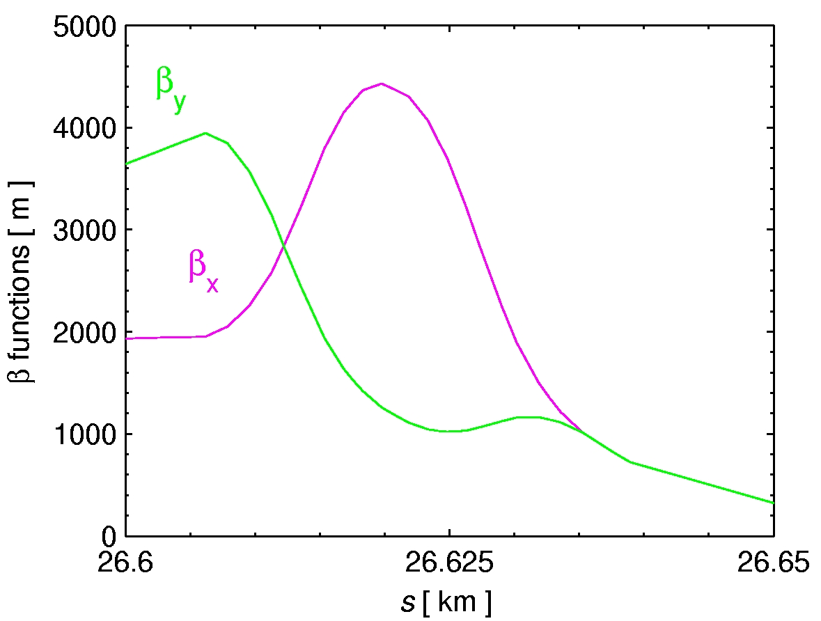
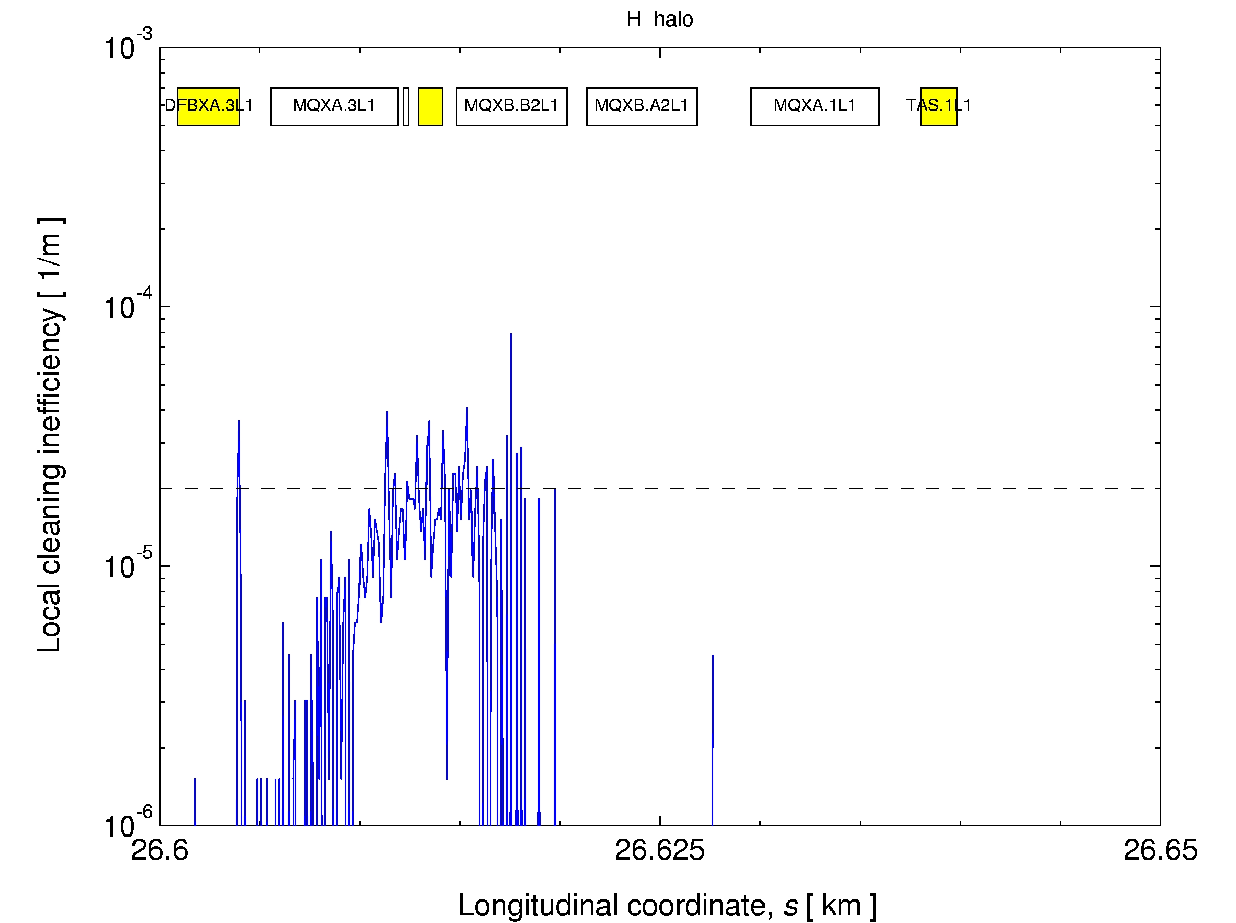
Transverse impact distributions at the triplet of IR Horizontal and vertical beta
functions (without TCT's!!). Longitudinal distribution of losses
(without TCT's!!). Transverse scatter plot of the
losses at the superconducting triplet of IR1 (without TCT's!!).
|
| |
|
|
|
Updated aperture model for optics version V6.500 [May 2006] Summary of recent changes of the aperture model:
In addition, the following minor changes were also implemented:
The status of the model was disussed at the ABP-LOC meeting of Feb. 14, 2006. See details in the slides presented by SR. In particular, note that the status of the warm elements and of the detector regions are not yet suitable for an automated extraction from the database into MADX format. The model is then still based on my scripts generated "manually" from the information collected from drawings and specification documents. An updated set of sources for BeamLoss Patterns is also available but it is not yet published on this page. If you need the new tools (that also work for beam 2!), contact directly the author (mailto SR). New aperture files (unzip with "gunzip2"):
Only the Twiss outputs are given here - the MADX source scripts are available on the AFS optics repository of V6.500.
Minor update (16/11/2007): manual correction of a couples of errors. The links to the Twiss have been updated. |
|
|
| Stefano Redaelli, Thursday, 05. April 2012 11:07 +0200 |